Extend LLMs Context Window

Introduction

A large context window is an absolutely desirable feature in Large Language Models (LLMs). However, enhancing these models’ abilities during pretraining period requires costly data collection and significant memory resources, which grow quadratically. Consequently, in the past year, large context window technology has become a highly contested field, drawing significant attention and debate. There are two desired properties: the input context length and the model output length. Generally, more focus is placed on the input context length, as few individuals, apart from those wishing LLMs to compose lengthy narratives, are interested in reading extensive output contexts.

Large context conditions are extremely important during the Retrieval-Augmented Generation (RAG) process because we aim for LLMs to read comprehensive materials and either output a perfect summary or utilize the key ideas from retrieved references. Indeed, while some models claim to read entire books, ongoing development has led to the expectation that, on the other hand, models be able to process a list of books, extensive tables, and more. Therefore, LLMs are on track to become an indispensable part of the workflow.

However, with limited resources at hand, most users are unable to retrain or fine-tune the models. Therefore, there is an urgent demand for creating resource-efficient adaptation and inference methods. These methods should ideally eliminate the need for retraining or supervised fine-tuning (SFT).

There are three sounds similar lines:

Length Extrapolation
Context Window Extension
Improving LLMs’ Utilization of Long Text

Previous Limitation

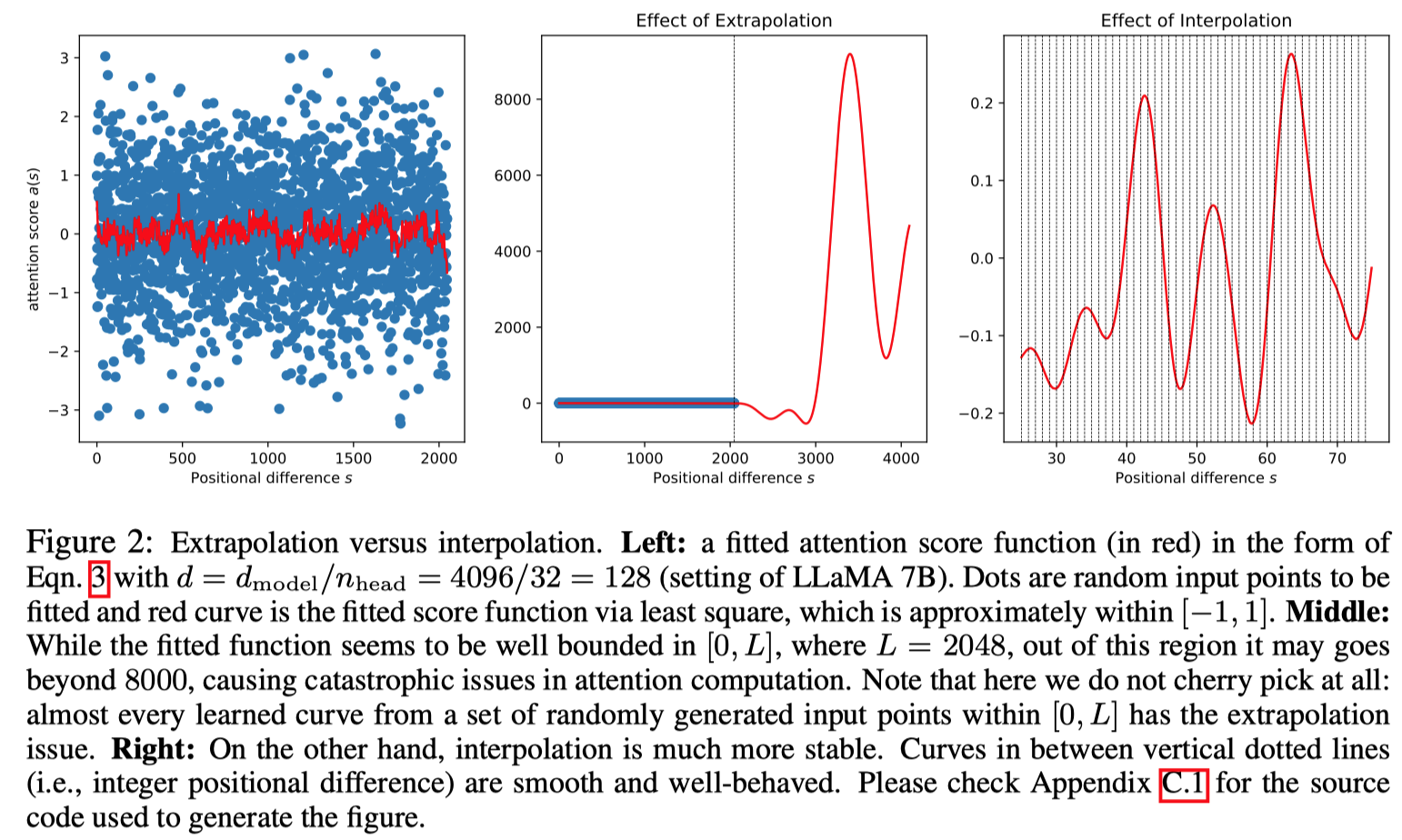
As demonstrated in the 📑Chen et al., 2023, they use coeffs linear fitting task show the abnormal attention amplitude appeared in the position exceed the pre-training context window size.

Methodology

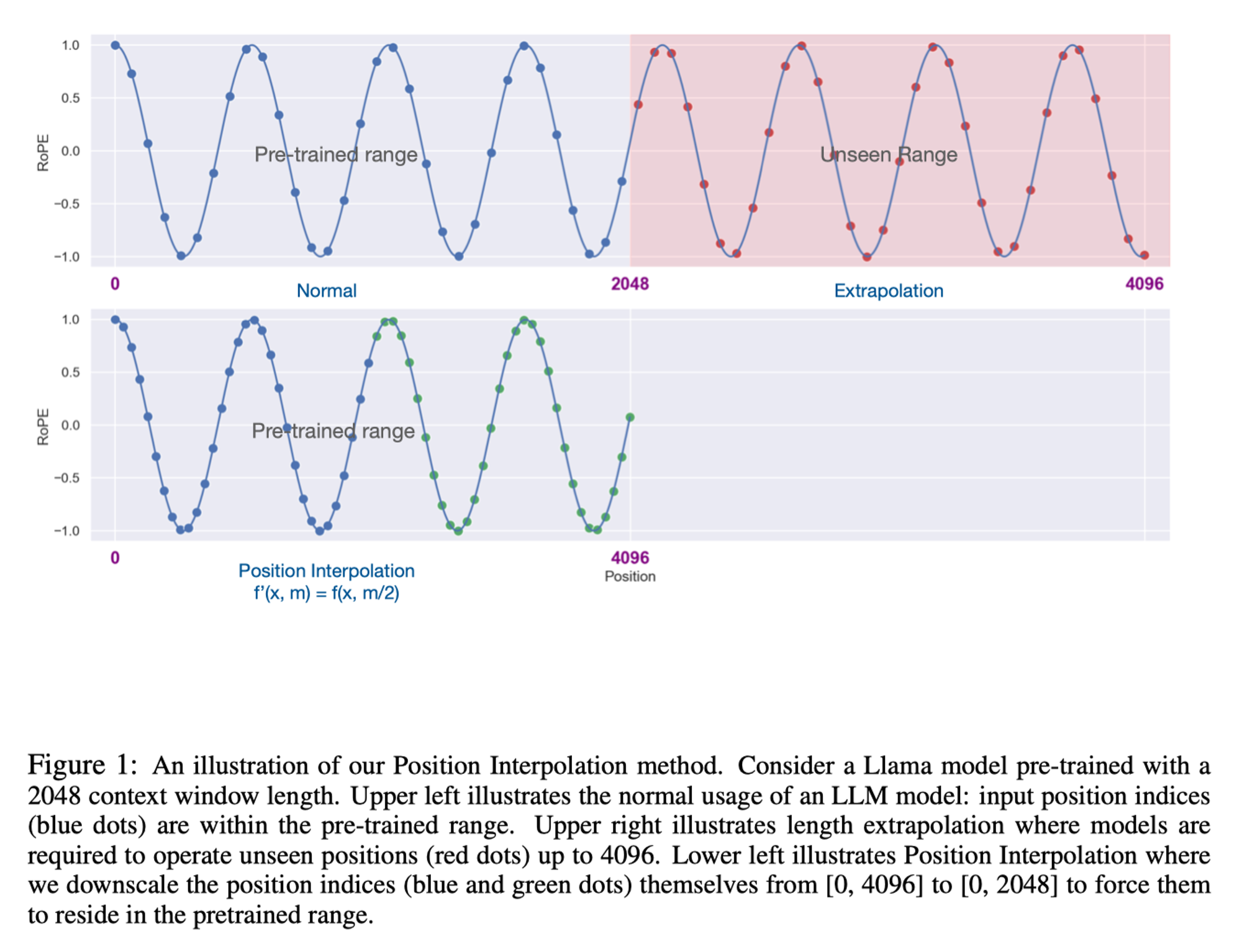
As what discussed in the 📑Chen et al., 2023, models often experience a catastrophic drop in performance when the input context window is directly extended. The root cause of this issue lies in the behavior of attention scores, which can become erratic due to encountering unexpected values—typically those exceeding the maximum context length used during the pretraining phase. This erratic behavior can lead to the generation of disproportionately large attention coefficients, thereby degrading the model’s representation capabilities. To mitigate this issue, 📑Chen et al., 2023 proposed an on-the-fly context re-distribution interpolation method that effectively prevents these abnormal jumps in attention scores:

\[\begin{equation} \mathbf{f}'(\boldsymbol{x},m)=\mathbf{f}\left( \boldsymbol{x},\frac{mL}{L'} \right), \end{equation}\]

Where \(L’\) represents the new maximum context window length. Using this scaling method, the position of each new input token can be accurately mapped into the original feasible numerical region, ensuring compatibility with the model’s pretrained structure.

Currently, no fine-tuning-free methods are available for this adjustment. However, LongRoPE 📑Ding et al., 2024 extends the context length by rescaling the RoPE positional encoding 📑Su et al., 2023 frequencies, allowing for a gradual extension of the context window. For a large language model (LLM) targeting a context window size of \(L’\) and processing a lengthy input document \(\boldsymbol{X}\),

\[\begin{equation} \mathop{\arg\min}_{\boldsymbol{x}\in \boldsymbol{X};\vert \boldsymbol{x}\vert \geq L'}\mathcal{L}(LLM(RoPE,\boldsymbol{X})) \end{equation}\]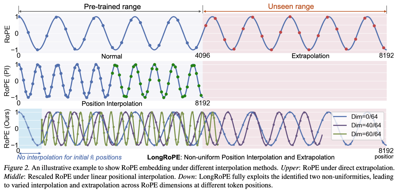

Given a position index \(m\in [0,c)\) and an embedding vector \(\boldsymbol{x}:=[x_{0}, x_{1}, \dots, x_{d-1}]^{\top}\), where \(d\) is the dimension of the attention head, RoPE 📑Su et al., 2023 defines a vector-valued complex function \(\boldsymbol{f}(\boldsymbol{x},m)\) as follows:

\[\begin{equation} \boldsymbol{f}(\boldsymbol{x},m)=[(x_{0}, ix_{1})e^{im\theta_{0}},(x_{2}, ix_{3})e^{im\theta_{1}},\dots,(x_{d-2}, ix_{d-1})e^{im\theta_{d/2-1}}]^{\top} \end{equation}\]

The self-attention score \(a(m,n)=\Re \langle \boldsymbol{f}(\boldsymbol{q},m),\boldsymbol{f}(\boldsymbol{k},n)\rangle =\dots =:a(m-n)\), thus enabling the effective use of the relative distance score equivalent in subsequent derivations.

Uniformly distribute the 4096 into 2048 position grids

As what they discussed in the 📑Chen et al., 2023, they dive into the detail of the position grids that interpolation between two grid \(s_{1}\) and \(s_{2}\) would not exceed an acceptable bound after fine-tuning on the larger corpus.

💡 How could catastrophic behaviors of ignoring information exceed the content length as attention score \(a_{m-n}\) decays, this distances should not matter that much?

It turns out that the upper bound derived in Section 3.4.3 of 📑Su et al., 2023 may be too loose: while it indeed decays with respect to \(\vert m-n\vert\), the bound can still be quite large (i.e., the bound can be critically depends on the magnitude of \(v_{j}\)) and thus vacuous.

\[\begin{equation} \boldsymbol{f}'(\boldsymbol{x},m)=\boldsymbol{f}\left(\boldsymbol{x},\frac{mL}{L'}\right) \end{equation}\]

Reason of bad performance brought by the direct interpolation

Let the attention score be denoted as \(a_{m-n}\), which indeed decays with respect to \(\vert m-n\vert\). If we consider all trigonometric functions as basis functions, (i.e., \(\phi_{j}(s):=e^{is\theta_{j}}\)):

\[\begin{equation} a(s)=\Re\left[ \sum^{d/2-1}_{j=0}h_{j}e^{is\theta_{j}} \right] \end{equation}\]

\(s\) represents the position between a query and key. The complex coefficients \(h_{j}:=(q_{2j}+iq_{2j+1})(k_{2j} - ik_{2j+1})\) depend on \(\boldsymbol{q}\) and \(\boldsymbol{k}\). When \(a(s)\) encounters an unexpected number (usually greater than 2048), it can exhibit unpredictable, abnormal behavior, i.e., output an extremely large coefficient. This negatively impacts the model’s representation capabilities.

💡 Theorem 2.1 (Interpolation bound). For attention score \(a(s) = \Re\left[\sum^{d/2-1}_{j=0}h_{j}e^{is\theta_{j}} \right]\), where \(\theta_{j}=c^{-2j/d}\), its interpolation value \(a(s)\) for \(s\in [s_{1}, s_{2}]\) is bounded as follows \(\begin{equation} \vert a(s)-a_{\rm linear}(s)\vert \leq d\left(\max_{j}\vert h_{j}\vert \right)\frac{(s-s_{1})(s_{2}-s)}{8\ln c} \end{equation}\) where \(a_{\rm linear}(s)\) is the linear interpolation of two grid point \(a(s_{1})\) and \(a(s_{2})\) that are known to behave well, enforced by LLM pre-training: \(\begin{equation} a_{\rm linear}(s):=(1-\lambda(s))a(s_{1})+\lambda(s)a(s_{2}),\quad \lambda(s):=\frac{s-s_{1}}{s_{2}-s_{1}} \end{equation}\)

This result ensures that the pre-trained LLMs maintain stable behavior, as their attention does not abruptly shift between grid points \(s_{1}\) and \(s_{2}\). Consequently, this approach achieves a condition where attention scores vary smoothly without causing chaotic amplitude fluctuations.

Fine-tuning

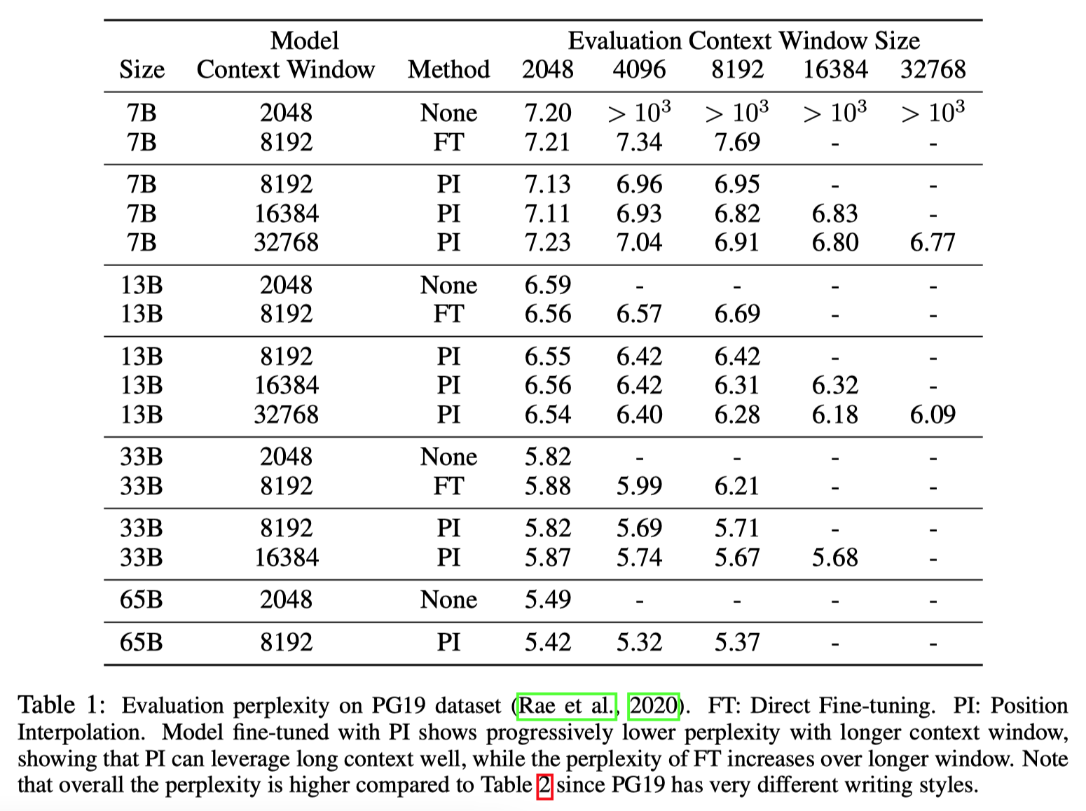
The interpolated model using the the next token prediction task with interpolated position encodings on the extended window size using a pre-training corpus such as the Pile.

Training Procedure:

AdamW with \(\beta_{1}=0.9\) and \(\beta_{2}=0.95\).
linear learning rate warmup of 20 steps starting from \(10\%\) maximum learning rate.
7B and 13B models, LR = \(2\times 10^{-5}\)
33B and 65B, LR = \(10^{-5}\)
weight decay: 0
batch size: 64

More GPUs are required for the large memory needed of large context.

Further discussion

https://www.reddit.com/r/LocalLLaMA/comments/14fgjqj/a_simple_way_to_extending_context_to_8k/

https://github.com/ggerganov/llama.cpp/discussions/1965

Infinite-length inputs LLMs

📑Xiao et al., 2024 were the first to discover that using an initial token as a placeholder can significantly enhance LLM performance in extremely large contexts, even if the placeholder token does not carry any meaningful information. Although this phenomenon appears counterintuitive to our expectations, it has proven to be effective.

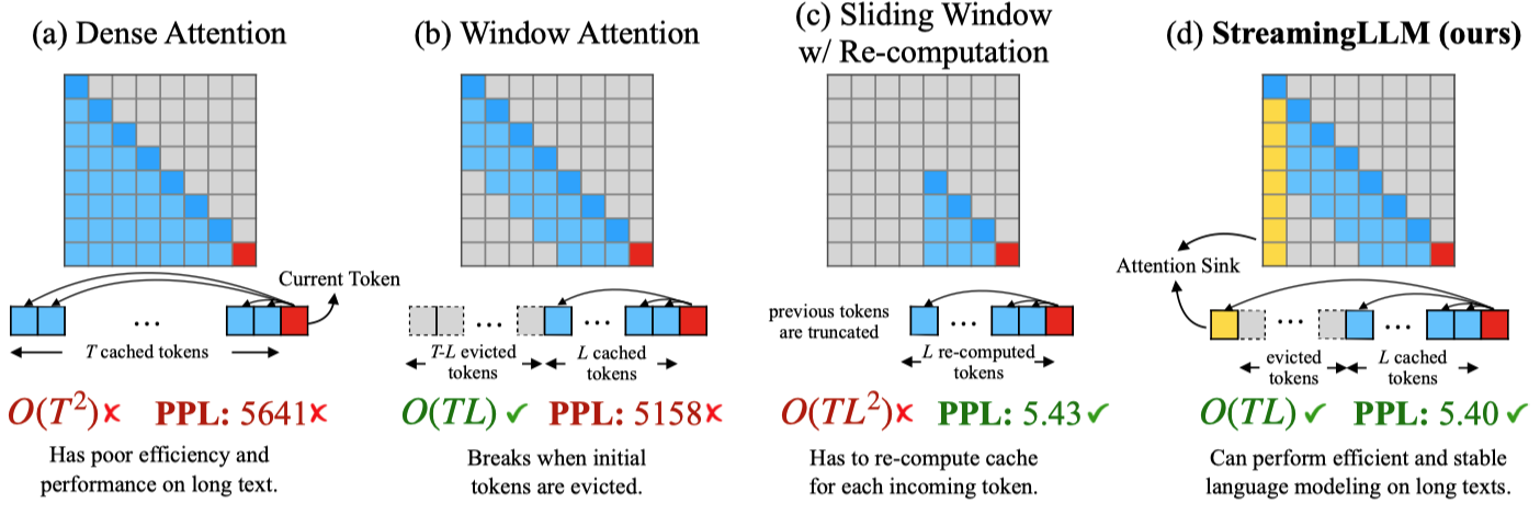
There are two hypothesis that:

Either initial tokens’ semantics are crucial;
the model learns a bias towards their absolute positions;

As attention score is computed by:

\[\begin{equation} \mathrm{Attention}(Q,K,V)=\mathrm{Softmax}\left( \frac{QK^{\top}}{\sqrt{d_{k}}} \right)V. \end{equation}\]

Consider any location in the sequence corresponding to this attention score matrix, such as the \(i\)-th elements. Let’s examine the attention scores associated with this position:

\[\begin{equation} \mathrm{Softmax}(x)_{i}=\frac{e^{x_{i}}}{e^{x_{1}}+\sum^{N}_{j=2}e^{x_{j}}},\quad x_{1}\gg x_{j}, j\in2,\dots, N, \end{equation}\]

as you can see, this \(e^{x_{1}}\) would appeared in every later token’s attention scores, it is emmm, almost a constant value. So, why not just make it a true constant value, thereby adapted function looks like:

\[\begin{equation} \mathrm{Softmax}_{1}(x)_{i}=\frac{e^{x_{i}}}{1+\sum^{N}_{j=1}e^{x_{j}}},\quad x_{1} \gg x_{j},j\in 2,\dots, N, \end{equation}\]

Note that \(j\) starts at 1, with the placeholder token serving solely to absorb unnecessary attention. This formulation does not require the attention scores for contextual tokens to sum to one. By substituting the original softmax function with this modified version, softmax1, the performance degradation remains within acceptable limits.

A explanation can be:

Consequently, the model tends to dump unnecessary attention values to specific tokens.

📌 Extensive research has been done on applying LLMs to lengthy texts, with three main areas of focus: Length Extrapolation, Context Window Extension, and Improving LLMs’s Utilization of Long Text. While seemingly related, it’s worth nothing that progress in one direction does’t necessarily lead to progress in the other. This paper does not expand the attention window size of LLMs or enhance the model’s memory and usage on long texts.

Therefore, we can recall the beginning hypothesis, if the initial token absorb most attention scores? The answer can be:

The initial tokens’ semantics are crucial ❌
The model learns a bias towards their absolute position ✅

Evaluation

Needle-in-a-Haystack test

Place a random fact or statement (the ‘needle’) in the middle of a long context window (the ‘haystack’)
Ask the model to retrieve this statement
Iterate over various document depths (where the needle is placed) and context lengths to measure performance

Passkey retrieval

In this task, the models are asked to recover a random passkey hidden in a long document. If a model consistently succeeds in retrieving the correct passkey value, means that effective context window size of the model is at least \(k\).

Long document summarization

There are list of datasets for this evaluation like GovReport, each document comes with a human generated summary. Use ROUGE-1/ROUGE-2/ROUGE-L scores to evaluate the models’ outputs vs the ground-truth summaries.

Counting stars

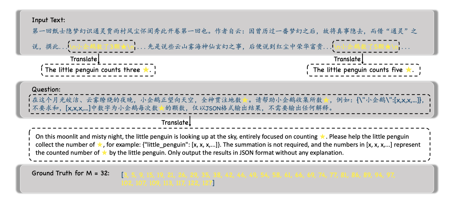
It seems this task lead to a more complex evaluation. Counting-Stars test refers to scattering multiple stars (sentences describing the number of stars) in the sky (a 128K long context), requiring LLMs to collect and summarize them into a specified answer.

Conclusion

Position Interpolation can effectively extend the context window of LLM models with minimal fine-tuning. The discovery that the “attention sink” plays a critical role in preserving the model’s ability to handle long context windows without performance degradation is particularly noteworthy. This area presents significant opportunities for further exploration.