iDAG
Invariant DAG Searching for Domain Generalization
Abstract
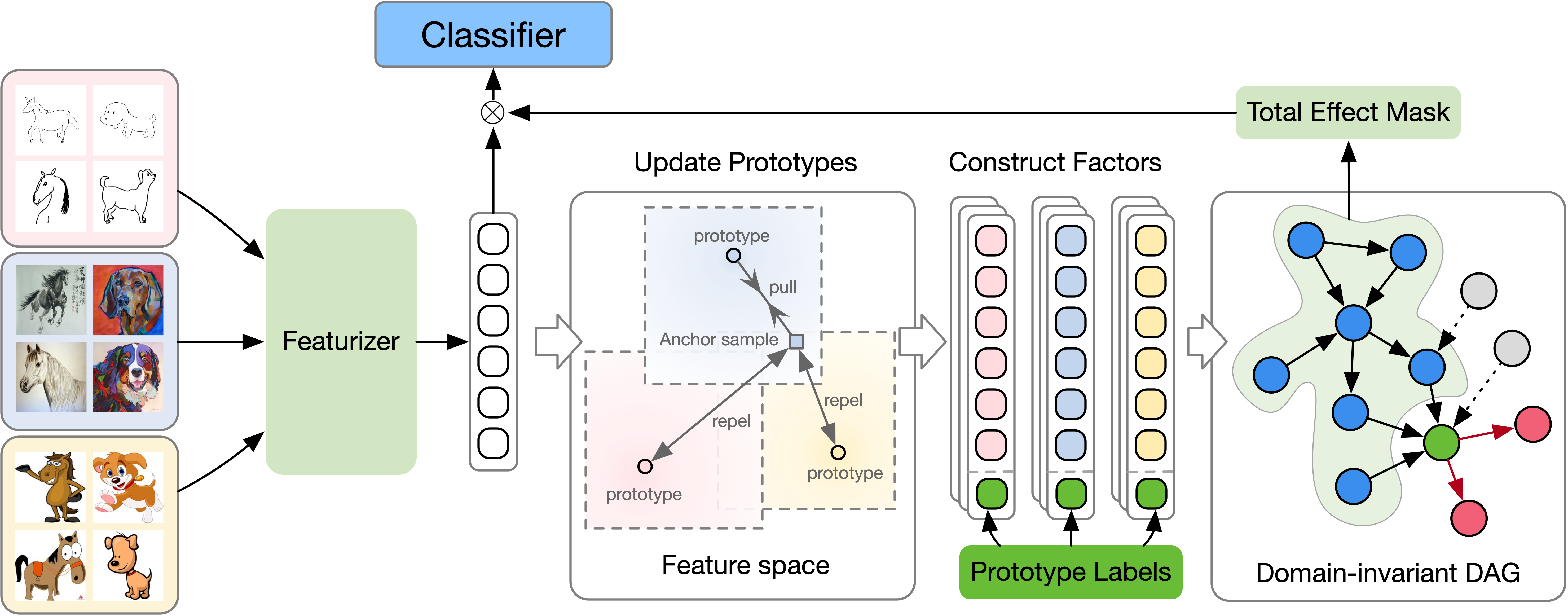
Existing machine learning (ML) models are often fragile in open environments because the data distribution frequently shifts. To address this problem, domain generalization (DG) aims to explore underlying invariant patterns for stable prediction across domains. In this work, we first characterize that this failure of conventional ML models in DG attributes to an inadequate identification of causal structures. We further propose a novel invariant Directed Acyclic Graph (dubbed iDAG) searching framework that attains an invariant graphical relation as the proxy to the causality structure from the intrinsic data-generating process. To enable tractable computation, iDAG solves a constrained optimization objective built on a set of representative class-conditional prototypes. Additionally, we integrate a hierarchical contrastive learning module, which poses a strong effect of clustering, for enhanced prototypes as well as stabler prediction. Extensive experiments on the synthetic and real-world benchmarks demonstrate that iDAG outperforms the state-of-the-art approaches, verifying the superiority of causal structure identification for DG.
Motivation

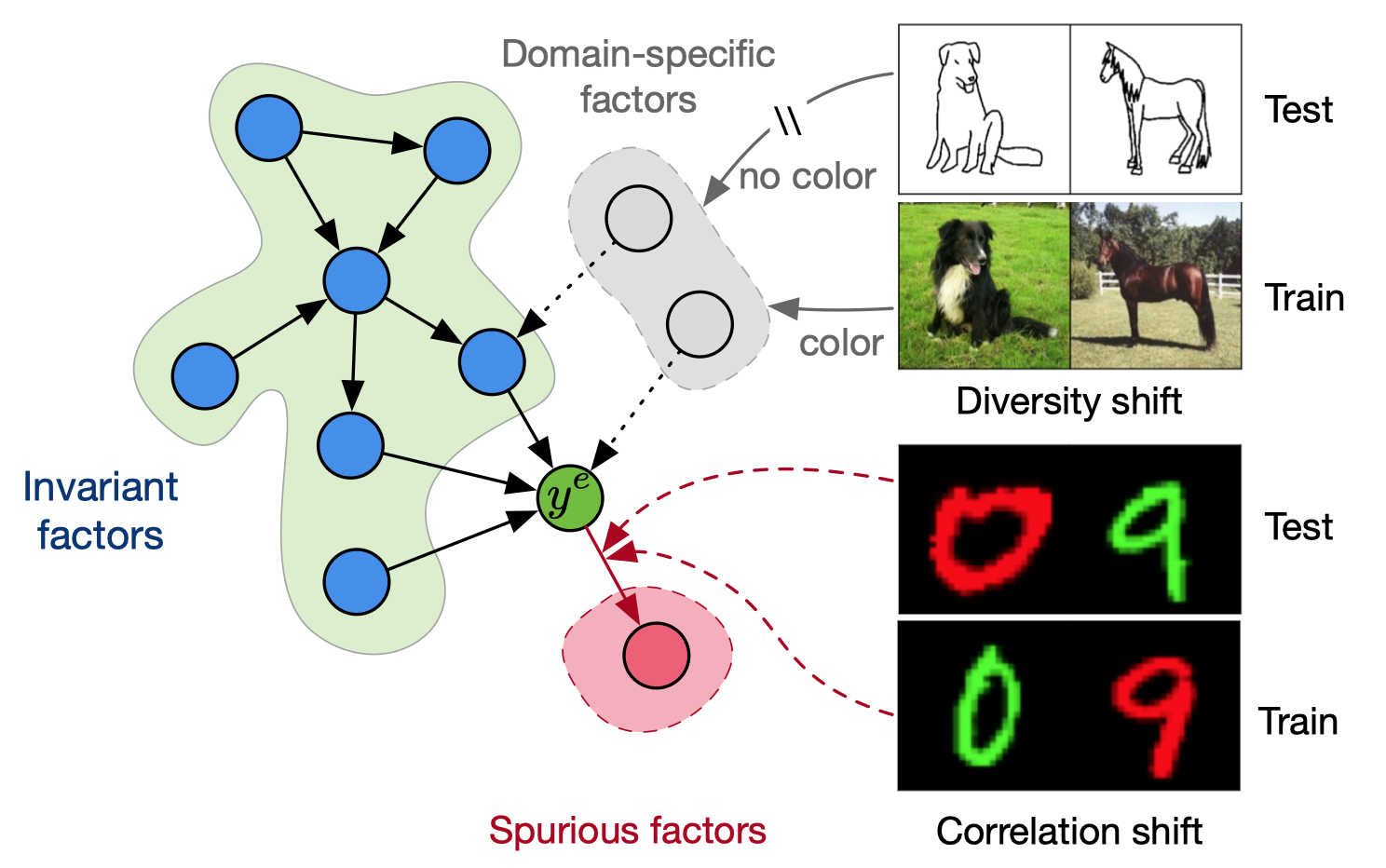
Data-generating process
Domain Generalization. The goal of domain/out-ofdistribution generalization is to explore the invariant pattern from multi-domain data to mitigate potential domain shifts when testing.
There is a group of injective data-generating functions \(g^{e}_{y}(\cdot), g^{e}_{s}(\cdot), g^{e}_{r}(\cdot)\), or each environment, the underlying factors of observational data follow the rule:
\[\begin{equation} y^{e}=g_{y}(\boldsymbol{z}^{e}_{y})+\epsilon_{y},\quad \boldsymbol{z}^{e}_{s}=g_{s}(y^{e})+\boldsymbol{\epsilon}^{e}_{s},\quad \boldsymbol{z}^{e}_{r}=\boldsymbol{\epsilon}^{e}_{r}, \end{equation}\]where \(\boldsymbol{z}^{e}_{y}\) denotes invariant features, \(\boldsymbol{z}^{e}_{s}\) denotes the easier-to-fit spurious features, \(\boldsymbol{z}^{e}_{r}\) denotes the domain-private features, \(\boldsymbol{\epsilon}^{e}_{y}\), \(\boldsymbol{\epsilon}^{e}_{s}\), \(\epsilon^{e}_{r}\) are mutually independent exogenous noises.
Stable DAG for Domains
For the sake of notational simplicity, we will use \(v_{i}\) to uniformly represent feature element \(z_{i}\) and label \(y\). Thereafter, we can define a structural causal model (SCM) on the whole collection of causal factors \(\mathcal{V}=\{v_{i}\}^{d}_{i=1}=\{z_{i}\}^{d}_{i=1}\cup \{y\}\).
Definition 1. (Domain Invariant DAG). A domain-specific SCM \(\mathcal{M}^{e}\) on a set of nodes \(\boldsymbol{V}^{e}\) with joint distribution \(p(\boldsymbol{v}^{e})\), according to Markov condition, it can be factorized by:
\[\begin{equation} p_{\mathcal{M}^{e}}=\prod_{i}p_{\mathcal{M}^{e}}(v^{e}_{i} | \textbf{Pa}^{e}_{i}) \end{equation}\]
Once the causal graph is reconstructed, the relations/factors of the task is determinined. (Please see the paper for details.)
iDAG

DAG
Let \(\boldsymbol{V} \in \mathbb{R}^{d\times n}\) be the values matrix of a set of vertices \(\mathcal{V}\), and \(\boldsymbol{v} \sim \mathcal{N}(0, \boldsymbol{\Sigma})\) (without the loss of generality, we assume the values are preprocessed by a simple bias term with zero means). The linear DAG model is given by:
\[\begin{equation} \boldsymbol{V} = \boldsymbol{A}^{e} \boldsymbol{V} + \boldsymbol{N} \end{equation}\]Therefore, we can find the causal graph by exploring the joint distribution of \(\boldsymbol{V}\):
\[\begin{equation} \mathcal{L}_{\rm rec}(\boldsymbol{A}^{e};\boldsymbol{\Sigma})=\frac{1}{2}\mathrm{Tr} \left((\boldsymbol{I} - \boldsymbol{A}^{e})^{\top}\boldsymbol{\Sigma}(\boldsymbol{I} - \boldsymbol{A}^{e})\right). \end{equation}\]The optimization problem is:
\[\begin{equation} \min_{\boldsymbol{A}^{e}} \mathcal{L}_{\rm rec}(\boldsymbol{A}^{e};\boldsymbol{\Sigma}) \quad \text{s.t.} \quad h(\boldsymbol{A}^{e})= e^{\boldsymbol{A}^{e}\odot \boldsymbol{A}^{e}} = 0 ~ (\boldsymbol{A}^{e} \in \mathrm{DAG}) \end{equation}\]Stable Feature Mask
To obtain a more stable prediction, it is required to collect not only the parent factors but also the ancestral factors of \(y\) in the DAG. Thus, we define invariant features by including all direct and indirect causal factors. Follow the idea of the fact that the positivity of the \((i,j)\) element of the \(k\)-th power of \(\boldsymbol{A}\) indicates the existence of a length-\(k\) path \(v_{i}\to \cdots \to v_{j}\), we derive the \(\boldsymbol{P}^{\text{tol}}\) to analogy the directed pairwise total effects,
\[\begin{equation} \boldsymbol{P}^{\text{tol}}=\left[\sum^{\infty}_{k=0}\frac{1}{k!}(\boldsymbol{A}\odot \boldsymbol{A})^{k} \right]=e^{\boldsymbol{A}\odot \boldsymbol{A}} \end{equation}\]Then, the invariant features \(\boldsymbol{z}^{e}_{y}:=\boldsymbol{z}^{e}\odot [\boldsymbol{P}^{\text{tol}}]^{\top}_{d+1,1:d}\in\mathbb{R}^{d}\) contains all the direct and indirect causal features of \(y\).